14 Ray Marching

14.1 Introduction

In traditional ray tracing, we cast rays from the camera through each pixel and determine their intersection with objects in the scene. The color at each intersection is calculated by considering lighting, material properties, and shadows.

Ray tracing excels at rendering reflective, refractive, and shadowed surfaces, creating highly realistic Images/raymarch.

However, ray tracing has its limitations when dealing with complex volumetric effects, implicit surfaces, or certain scenes where geometry isn’t explicitly defined by polygons. In such cases, the point of intersection between a ray and a surface may not be easily computed, or the surface itself may not be well-defined, such as in the case of clouds, fog, or fractals.

14.2 Introducing Ray Marching

To overcome these challenges, we introduce ray marching. Unlike ray tracing, where we compute precise intersections between rays and surfaces, ray marching samples the scene at different intervals along the ray’s path. This technique is particularly useful for rendering volumetric media and distance fields.

Ray marching works by “marching” a ray through the scene, advancing step by step, and evaluating the properties of the scene at each sample point. There are many form of ray marching, and they differ mainly in how they determine the step size and when to stop marching. In this chapter, we will discuss the main applications of ray marching, including implicit surfaces, signed distance fields, and volume rendering.

14.3 Implicit Surfaces and Signed Distance Fields

In Chapter 8, we introduced geometries using polygons and meshes. This kind of representation is explicit, meaning that we specify exactly the shapes and surfaces that make up the scene using vertices and triangles. This form of representation is intuitive and easy to work with. However, it can be limiting when dealing with complex organic shapes that require a large number of polygons to approximate accurately.

On the other hand, implicit surfaces are defined by mathematical functions that describe the surface’s properties without explicitly defining the surface itself. Signed distance fields (SDFs) are a common way to represent implicit surfaces.

An SDF is a scalar field that assigns a distance value, either negative or positive, to each point in space, indicating the closest distance to a surface. A point inside the surface has a negative distance, while a point outside the surface has a positive distance, and points on the surface have a distance of zero.

This representation allows us to describe complex shapes and surfaces using simple mathematical models, create smooth and continuous surfaces.

Consider the following SDF in 2D:

\[ d(p) = \sqrt{p.x^2 + p.y^2} - r \]

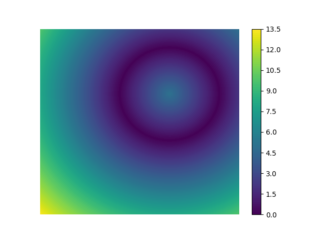
where \(p\) is the point in space. If we plot out the distance field, we get a circle of radius \(r\) centered at the origin. In other words, this SDF describes a circle with radius \(r\).

The field below is that function, evaluated everywhere and coloured by the value it returns. Move the pointer around it: the dashed circle is the largest circle you could draw at that point without touching the surface, and its radius is exactly the number the function gave back.

By combining multiple SDFs and applying operations like blending, union, and intersection, we can create complex shapes and surfaces that are difficult to represent explicitly with polygons.

Each of those operations is a single line of arithmetic on the two distances. Try the smooth union in particular, and drag its blend radius \(k\) — filleting two shapes together is a hard problem for meshes and a one-parameter problem here:

SDFs are particularly well-suited for ray marching, as they provide a natural way to compute the distance to the nearest surface along a ray’s path.

14.3.1 Sphere Tracing

Let us reconsider the problem of ray-object intersection: at any point in space, we can cast a ray in any direction and evaluate the SDF to determine the distance to the nearest surface. This distance is then used to “march” the ray through the scene, advancing step by step until we reach the surface or a maximum distance threshold. If the ray reaches the surface, then we have an intersection point. Note that this ray-object intersection does not require explicit geometry or polygons; it is based on the SDF function that describes the surface.

By making no changes to the direction and always taking steps sizes equal to the distance to the nearest surface, we can guarantee that the ray will never miss the surface. Intuitiivly, regardless of the ray’s initial position or direction, if the step taken is not longer than the distance to the nearest surface, then the ray will never “jump” over the surface.

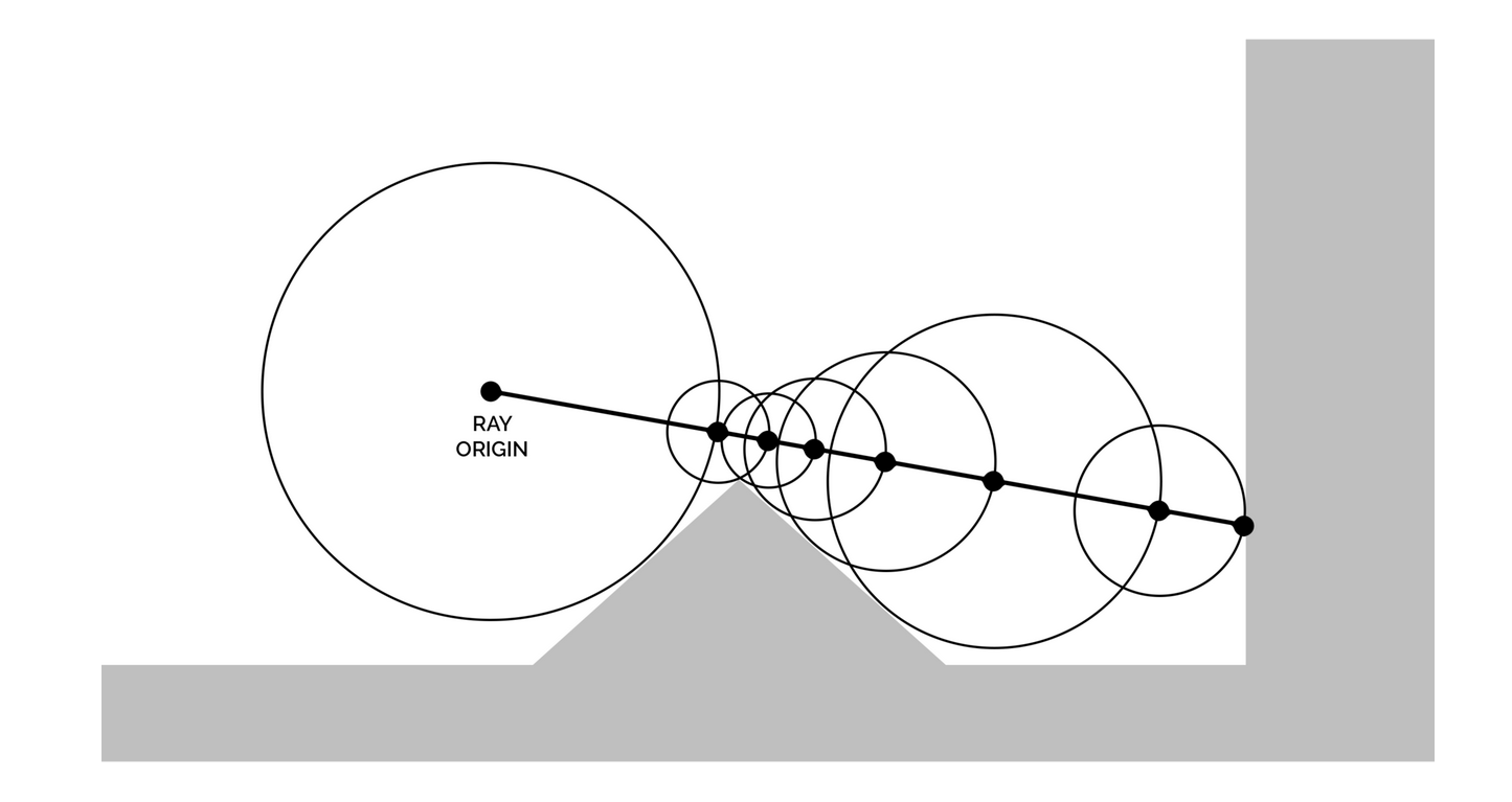
Press Step below to advance the ray one iteration at a time. Each circle is the empty space the SDF has just guaranteed, and the circles touch end to end — which is the geometric argument that nothing was skipped. Then push the step multiplier above 1.0 and watch the guarantee break:

We can extend this idea to 3D by casting a ray from the camera through each pixel and marching it through the scene, evaluating the SDF at each step, and moving towards the nearest surface.

This process is known as sphere tracing, as it involves tracing a sphere of radius \(r\) along the ray’s path, where \(r\) is the distance to the nearest surface. The sphere is moved along the ray’s path until it intersects the surface, at which point we have found the intersection point.

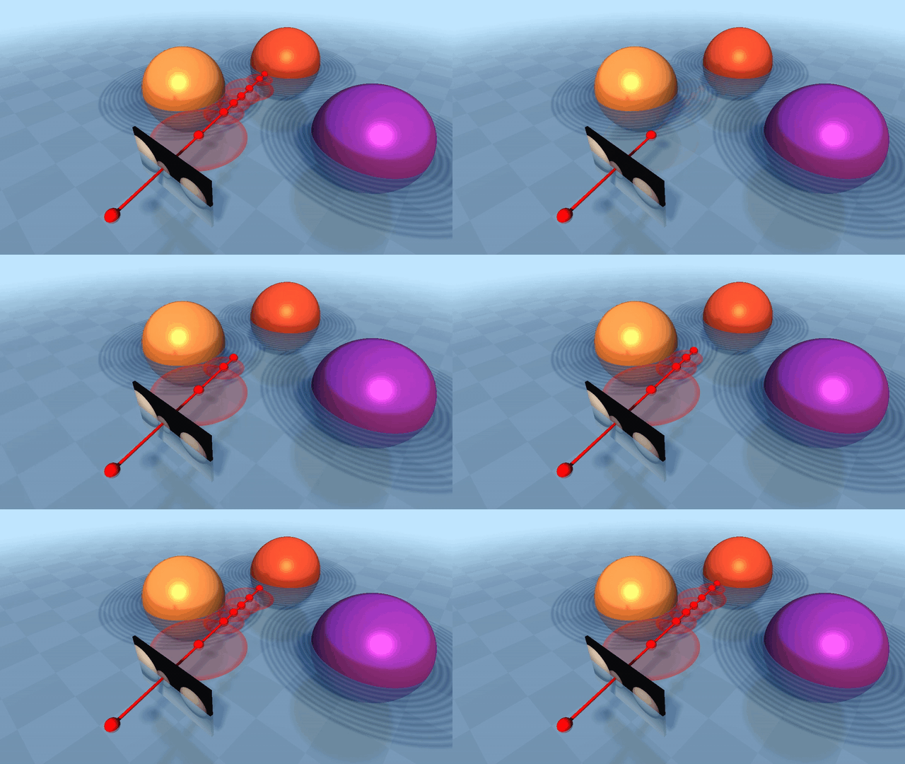
The complexity of the scene is determined by the SDFs used to represent the objects. By combining simple SDFs and applying operations like blending, union, and intersection, we can create complex scenes with smooth surfaces and intricate shapes. We can even model fractals, clouds, and other volumetric effects using SDFs.

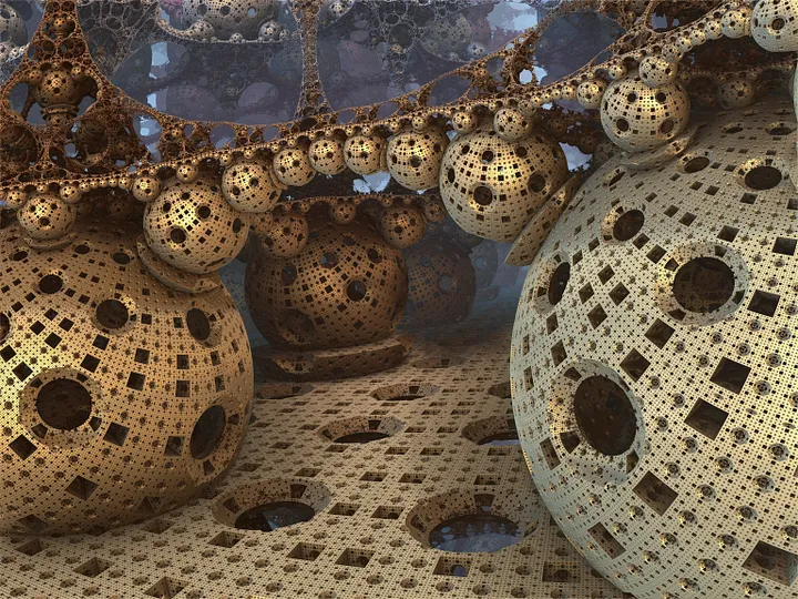
The Mandelbulb fractal, is an intricate 3D fractal that can be represented using an SDF and rendered using sphere tracing. (More on the Mandelbulb)

The scene below is running that loop for real, once per pixel, in a fragment shader. There is no geometry on the page at all — no vertices, no triangles, no model file — only the ten-line distance function shown beside it. Switch to the cost view to see how many iterations each pixel actually needed:

Because SDFs are mathematical functions, we can numerically compute their gradients, which allows us to calculate surface normals for shading and lighting as well, in which case, we can apply the same techniques we used in ray tracing to render the scene.

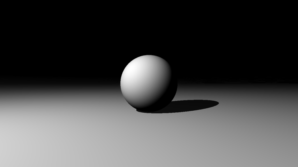
That gradient is computed by sampling the field a hair to either side of the hit point and asking which way the distance grows fastest. The whole thing rests on the size of that offset \(h\), and it fails in two opposite ways — try it at both extremes:

14.4 The Physics of Light in Volumetric Media

Another application of ray marching is volume rendering, which involves rendering volumetric effects that beyond what can be achieved with traditional ray tracing, these include clouds, fog, smoke, and other media that are not easily represented by explicit geometry and requires modelling more complex light interactions, such as scattering and absorption.

In the previous chapter, we modelled light rays as straight lines that carry radiant energy and interacts with surfaces by reflecting, refracting, and absorbing light.

In the case of volumetric media, light interacts with the individual particles in the medium that scatter and absorb light. To model this interaction, we need to consider the following:

14.4.0.1 Absorption

When light enters a medium, e.g., clouds that consists of water particles, it is absorbed by the particles, causing the light to lose energy as it passes through the medium, thus reducing the radiance as it passes through. This one of the reasons why it is much darker on a cloudy day than on a clear day, as the clouds absorb and scatter the sunlight, reducing the amount of light that reaches the ground.

In addition to absorbtion, light rays are also scattered in all directions by the particles in the medium, similar to how light would reflect of a solid surface, and only a portion of the light reaches the observer.

This scattering is responsible for the diffusion of light in the medium, creating a soft, hazy appearance, and is what gives clouds, fog, and smoke their characteristic look.

Scattering can be divided into two types: out-scattering and in-scattering.

14.4.0.2 Out-scattering

Out-scattering occurs when a light ray, \(\omega_i\) that is travelling towards the observer, enters the medium and is scattered by the particles in the medium in another direction \(\omega_o\). Radiance decreases.

14.4.0.3 In-scattering

In-scattering occurs when a separate light ray, \(\omega_s\) that was not originally travelling towards the observer, is scattered by the particles in the medium and redirected towards the observer. Radiance increases.

14.4.0.4 Emission

To complete the model, we also consider emission, where the medium itself emits light, such as in the case of fire, lava, or other light sources within the medium.

In this case, the medium emits light in all directions, contributing to the overall radiance of the scene, including the light that reaches the observer.

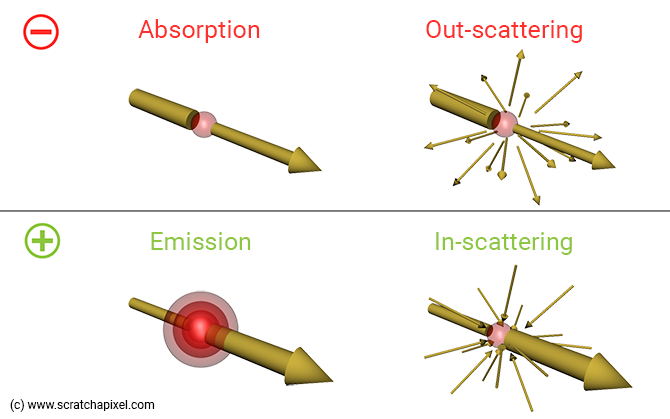
All four are switchable below. The photons show you the mechanism; the curve beside them shows the consequence for radiance. Pay particular attention to what happens when you swap absorption for out-scattering — the photon counters tell two completely different stories, and the curve cannot tell them apart:

Combining these four interactions, we can derive a simple model of the change in radiance as light passes through a medium:

\[ dL(p, \omega) = \text{emission}+ \text{in-scattering} - \text{out-scattering} - \text{absorption} \]

where: - \(dL(p, \omega)\) is the change in radiance at point \(p\) within the medium in the direction \(\omega\).

All these interaction occur at a molecular level. To model this realistically, we would need to simulate the interactions of billions of particles in the medium, which is computationally infeasible.

Instead, we simplify these interactions by modelling these interactions probabilistically, similar to how we model light interactions with surfaces in ray tracing.

In other words, we consider the probability of light being absorbed or scattered. A medium that is less likely to absorb or scatter light would appear more transparent and let more light through, such as the case of mist, while a medium that is more likely to absorb or scatter light would appear darker and more opaque, such as the case of smoke.

14.4.1 Coefficients of Absorption and Scattering

To model the absorption and scattering of light in a medium probabilistically, we use coefficients that describe how light interacts with the medium. These coefficients are defined as follows:

14.4.1.1 Absorption Coefficient

The absorption coefficient, \(\sigma_a\), describes the probability of light being absorbed by the medium as it passes through. A higher absorption coefficient means that light is more likely to be absorbed, resulting in a darker appearance.

14.4.1.2 Scattering Coefficient

The scattering coefficient, \(\sigma_s\), is similar to the absorption coefficient but describes the probability of light being scattered in all directions.

14.4.1.3 Extinction Coefficient

From the persective of the observer, the effect of out-scattering and absorption have on the radiance is indistinguishable. In other words, the observer cannot tell whether the light was absorbed or scattered, instead, they only see the total reduction in radiance.

Therefore we can combine the absorption and scattering coefficients into a single coefficient called the extinction coefficient, expressed as:

\[ \sigma_t = \sigma_a + \sigma_s \]

where \(\sigma_t\) is the total attenuation of light as it passes through the medium. This is also called the attenuation coefficient.

It is often useful to think of the coefficient as the density of particles in the medium, where a higher coefficient means more particles and a higher probability of light interacting with the medium.

14.4.2 Beer-Lambert Law

The Beer-Lambert Law describes how light is attenuated as it passes through a medium with absorption and scattering. In the simplest case, where the medium is homogeneous and isotropic, meaning that the absorption and scattering coefficients are constant throughout the medium, the Beer-Lambert Law is given by:

\[ L(d) = e^{-\sigma_t d} \]

where:

\(L(d)\) is the radiance at distance \(d\) into the medium.
\(\sigma_t\) is the extinction coefficient of the medium.
\(d\) is the distance the light has travelled through the medium.

For a medium with a non-constant extinction coefficient, we need to model something called transmittance, which describes the fraction of light that passes through the medium at a given distance \(d\). The transmittance is given by:

\[ T(d) = \exp\left(-\int_0^d \sigma_t(x) dx\right) \]

where: - \(T(d)\) is the transmittance at distance \(d\) into the medium. - \(\sigma_t\) is the extinction coefficient - \(d\) is the distance the light has travelled through the medium. - the integral represents the accumulation of the extinction coefficient along the path of the light ray from where it entered the medium to distance \(d\).

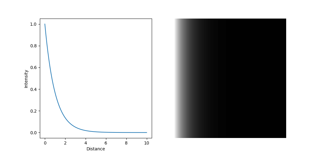
Without going into the details of the derivation of this law, we can Intuitiivly understand the meaning of it.

By plotting out the Beer-Lambert Law, we see that the radiance decreases exponentially as the light passes through the medium, with a steeper decline for higher extinction coefficients.

The panels below make the non-uniform case concrete. Draw any density profile you like on the top panel and the other three follow it: the optical depth accumulates the area underneath, the transmittance is what survives, and the strip at the bottom is that number rendered as light. Leave the profile flat and the integral collapses back to \(\sigma_t d\) — the simple formula is the special case:

For the interested reader, you can find the derivation of the Beer-Lambert Law here.

The Beer-Lambert Law, therefore, lets us calculate the amount of radiance we expect to see at a given distance into the medium, based on the absorption and out-scattering coefficients of the medium.

14.4.3 In-scattering and the Phase Function

Finally, we consider in-scattering, which is the notion that light can be scattered from other points in the medium towards the currect point, in the direction of the observer.

In-scattering is a very complex phenomenon that is difficult to model accurately. Instead, just like we’ve done with other complex light interactions, we model in-scattering probabilistically.

We want to model the probability of a light coming from an arbitrary direction, \(\omega^{\prime}\), being scattered towards the observer, \(\omega\), at some point in the medium \(p\).

This is very similar to the BRDF, which models the probability of light being reflected in a certain direction from a surface. In the context of volume rendering, this is called the phase function, expressed as:

\[ f_p(p, \omega, \omega^{\prime}) \]

and it outputs the probability of light coming from direction \(\omega^{\prime}\) being scattered towards the observer in direction \(\omega\) at point \(p\) in the medium.

The radiance produce by in-scattering is then given by: \[ L_s(p, \omega) = \int_{S^2} f_p(x, \omega, \omega^{\prime}) L(x, \omega^{\prime}) d\omega^{\prime} \] where:

\(L_s(p, \omega)\) is the radiance produced by in-scattering at point \(p\) in direction \(\omega\).
\(f_p(p, \omega, \omega^{\prime})\) is the phase function.
\(L(p, \omega^{\prime})\) is the radiance at point \(p\) from an arbitrary \(\omega^{\prime}\), note that this is a recursive definition, similar to the rendering equation in ray tracing.
the integral is over the hemisphere \(S^2\) of all possible directions \(\omega^{\prime}\).

Intuitively, this equation states that: the radiance produced by in-scattering in the direction of the observer, is the sum of the in-scattered radiance from all possible directions in the hemisphere, weighted by how likely each radiance is to be scattered in the direction of the observer.

Note that the in-scattered radiance is defined recursively, as it depends on the radiance from other points in the medium, in practice, the deeper the recursion, the more accurate the result, but also the more computationally expensive.

The exact form of the phase function depends on the medium and the type of scattering that occurs, but we will not go into the details of the phase function in this chapter.

The most common choice, Henyey-Greenstein, controls the entire shape of that distribution with a single number \(g\). Drag it from \(-1\) to \(1\) and watch the lobe swing from backwards to forwards — then move the sun behind the puff and raise \(g\) to see where a cloud’s silver lining comes from:

You may find more information about the phase function and its properties here.

14.5 The Volume Rendering Equation

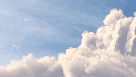
Piecing everything together, we can derive the volume rendering equation (VRE). The VRE describes how light interacts with a volume of a medium and how the radiance changes as light passes through the medium. The VRE, with abuse of notation, is given by:

\[ L = \int_{t=0}^{d} T(t)[ \sigma_s L_s+ \sigma_a L_e] dt + L(0) T(d) \]

where:

\(L\) is the radiance at the observer
\(T(t)\) is the transmittance at distance \(t\) into the medium
\(\sigma_s\) is the scattering coefficient
\(L_s\) is the radiance produced by in-scattering
\(L(0)\) is the radiance at the entry point of the medium
\(T(d)\) is the transmittance through the entire medium

Here, we’ve simplified the notation of the VRE to make it easier to understand, the VRE can be intuitevly understood as follows:

The first term represents the radiance produced by in-scattering and emission as light passes through the medium.
At every point in the medium, in-scattering and emission may occur and contributes to the radiance, so we need to integrate over the entire path of the light ray to accumulate the radiance produced by in-scattering and emission.
But at the same time, the radiance produced by in-scattering and emission may be absorbed or scattered out of the medium, so we need to account for that loss through the transmittance \(T(t)\), i.e. the fraction of light that passes through the medium at distance \(t\).
The second term represents the radiance at the entry point of the medium, i.e. what comes through from behind the medium. This is attenuated by the transmittance \(T(d)\), meaning that we only see a fraction of the radiance that enters the medium.

14.6 Ray Marching for Volume Rendering

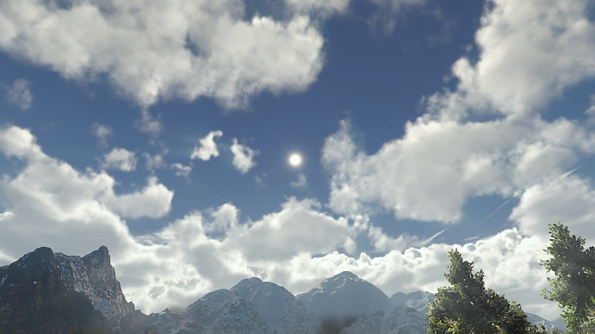
The VRE involves integrating over the entire path of the light ray through the medium, following the direction of the ray. There is a problem with this approach: the integral in the VRE is continuous, meaning that we need to evaluate the radiance an infinite number of times along the path of the light ray. This is computationally infeasible.

To address the challenge, we use ray marching to compute the interaction of light with the medium at discrete intervals along the path of the light ray. The step size of the ray marching determines the accuracy of the result, with smaller steps providing more accurate results but requiring more computation. The discretised VRE is then given by:

\[ L = \sum_{i=0}^{n} T(t_i)[ \sigma_s L_s+ \sigma_a L_e] \Delta t_i + L(0) T(d) \]

and

\[ T(t) = \exp\left(-\sum_{j=0}^{i} \sigma_t(x_j) \Delta x_j\right) \]

where: - \(\Delta t_i\) is the step size of the ray marching

Here, we’ve simply converted the continuous integral into a discrete sum, where we evaluate the radiance at each step of the ray marching. The transmittance \(T(t)\) is also computed at each step, accumulating the extinction coefficient along the path of the light ray.

The cost of that approximation is visible directly. Below, the same volume is rendered twice — on the left with the step count you choose, on the right with a fine reference — and the plots underneath show the rectangles your sum is actually using. At low step counts the sum invents structure that is not in the volume: banding across smooth gradients, and a regular lattice of false detail wherever the density has texture. Then tick jitter, which does not reduce the error at all but scatters it into noise the eye forgives:

14.6.1 Volume Density Field

There is one final piece of the puzzle that we need to consider to perform volume rendering: determining the probability density coefficent, or simply the density, of the medium at each point in space.

There are many ways to represent the density of a volume, but one common approach is to use a volume density field, which assigns a density value to each point in the volume. In practice, the density field is often represented as a 3D texture.

A 3D texture is similar to a 2D texture, but with an additional dimension, instead of sampling using 2D coordinates, \((u, v)\), we sample using 3D coordinates, \((x, y, z)\). Here, each texture element, or texel, contains a density value, between 0 and 1, that describes the density of the medium at that point in space. Formally, we can define the density field as:

\[ \sigma(p) : \mathbb{R}^3 \rightarrow \mathbb{R} \in [0, 1] \]

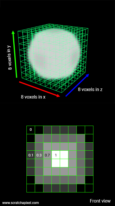
Scrub through the slices below to see what that stack of texels actually contains, and switch between nearest and trilinear filtering to see what the hardware blend is buying you. Drop the resolution to \(8^3\) and the texels become visible as cubes in the render — the volumetric version of a pixelated texture:

14.6.2 Volume Rendering Process

With the density field in place, we can now perform volume rendering using ray marching. The process is as follows:

Initialise a transimittance value \(T=1\), and a radiance value \(L=0\). This means that we start with full transmittance and no radiance. This makes sense Intuitively as 100% of the light before the medium would reach the observer, and there is no radiance produced by the medium yet.
Cast a ray from the camera through each pixel, this is called forward ray marching. Note that in ray tracing, we called this backward ray tracing. The terminology is the opposite, and it can be confusing. But the idea is the same, we cast rays from the camera through each pixel to determine the color of the pixel.;

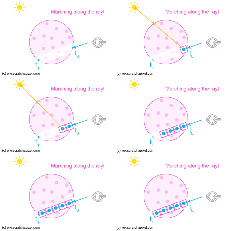
Side Note: Since there is forward ray marching, there is also backward ray marching, where we cast rays following the direction of the light ray, instead of the direction from the observer. We will not delve into backward ray marching in this chapter.

Find where the ray enters volume. This is counter intuitive, since volumes don’t have well-defined surfaces. Instead, we need to find where the ray enters and exits the bounding box of the volume. We do this so that we don’t waste computation on sampling empty space outside the volume.

That test is worth seeing on its own, because it is only a handful of comparisons and it decides how much work the rest of the algorithm does. Drag the ray past the box, then straight through it, then start it inside:

March the ray through the volume by taking fixed steps along the ray’s path.
- At each step, sample the density field to determine the density \(\sigma_t\) of the medium at that point and update the transmittance \(T=T \exp(-\sigma_t\Delta x)\), following the discretised VRE.
- Compute the radiance produced by in-scattering and emission at that point, \(L_s\) and \(L_e\), and accumulate it in the radiance \(L\), multiplied by the transmittance.
- In other words, we compute the radiance produced by the medium at each step and attenuate it by the transmittance, since for every step we take further into the medium, less light reaches the observer.
Repeat the ray marching until the ray exits the volume or reaches a maximum distance threshold.

Here is that entire loop, executed one step at a time. Watch the two accumulators: \(T\) starts at 1 and can only fall, \(L\) starts at 0 and can only rise, and every step adds its contribution multiplied by whatever \(T\) happened to be at the time. Note how few of the steps actually matter once \(T\) has dropped — which is exactly what the early-ray termination checkbox exploits:

14.7 Putting It All Together

Finally, everything in this chapter at once, running in real time: a bounding slab, a procedural density field, transmittance by Beer-Lambert, in-scattering weighted by a phase function, a second nested march toward the sun for shadowing, and early-ray termination paying for it all.

Every term has its own slider, including the ones that break it. The cost panel is worth watching as you move them — the nested light march is what makes volumetric rendering expensive, and dropping it to a single step will show you why real cloud renderers go to such lengths to avoid paying for it honestly.

13 Ray Tracing

15 Graphics in ML